
Evaporative airconditioners work by pulling outside air through wet sponges to reduce the air temperature before venting this air into the building. This is made possible by the cooling effects of evaporation and is goverened by environmental conditions. I have long wanted to apply some kind of automation or mathematical model to my air conditioner to run it more optimally on hot days.
After 5 years into the smart home journey, there is no lack of sensors around the house to record every aspect of the environment including temperature, humidity, atmospheric pressure, motion , power usage, and cameras.
I want to use this information to make smart decisions about how to run the airconditioner at the best fan speed on a day with a particular set of climate condisions. One speed might work great on a relatively dry day, but there is no guarantee it works the same on a different day, at a lower temperature and more moisture in the air.
Background
Evaporative cooling, it turns out, works best on hot, dry air because it is able to absorb more moisture (think of a dry sponge). Wet and humid air, on the other hand, acts more like a wet sponge unable to absorb more moisture. Not only is hot air able to evaporate more water, it is also able to hold more moisture compared to cool air. In other words, if you chill a cubic meter of hot air and reduce its temperature from 30 dgrees down to 5 degrees, you will find that water condenses from the air (like squeezing out a wet sponge)
For these reasons evaporative cooling works best when the climate is dry and hot, which would be ideal conditions. Evaporation is literally impossible when the relative humidty is 100% and its efficacy decreases dramatically as relative humidy approaches faily damp conditions. The lowest possible temperature an evaporative cooler can achieve is called the wet bulb temperature. Technology Connections on Youtube did a great job summarising this in their videos about Swamp coolers and air conditioning. See embedded video below up until approximately 20:30min.
Challenge of optimisation
We are obviously not in control of the weather (which presents 3 variables in this scenario), which sparked my interested in using an experimental approach. My AC is a basic model that can be controlled by increasing or decreasing the fan speed on a scale of 1 through to 10 settings. This is the variable we are able to adjust and ultimately I want the system to tell me which speed setting to use for maximim cooling effect given all of the environmental variables.
Other factors such as outdoor temperature, humidity and atmospheric pressure vary thorughout the day, however, for the duration of one experiment we can assume these to be constant (minor variation that is unavoidable).
The challenge is that throughout the day, the inputs change and so does the fan speed that produces the optimal output air temperature (this is my theory).
Manual Optimisation by running experiments
I want to be able to run the air conditioner fan at different speeds and have the system monitor for any changes in indoor temperature and humidty. The system records these results, and then requests speed adjustments to gather more data. Finally, it is able to recommend the optimal fan speed.
Automated Optimisation by classification/prediction
The system should use all the data collected during manual optimisations to create a predictive model. Given measurements for all input variables about the current environment, the system should run these through a machine learning classification algorithm which maps these inputs to the optimal fan speed. The table below shows an example. Given the data for $t=1$ and $t=2$, the system should be able to classify the inputs for $t=n$ and map them to a fan speed.
| Time | Variables | Best Fan Speed |
|---|---|---|
| $t=1$ | $$T_o = 35C, H_o = 60%, A=1002mb$$ | 6 |
| $t=2$ | $$T_o = 20C, H_o = 40%, A=998mb$$ | 3 |
| $t=n$ | $$T_o = 38C H_o = 75% A=1005mb$$ | ? |
How to measure cooling efficiency
In order to measure the air conditioners efficiency at any given time we need a to come up with a metric. I have previously published a custom component for Home Assistant called Meteorologic Metrics and another one Cooler Efficiency which collect environmental climate conditions and calculate a series of values to be used in the analyis.
I have made two more custom components for Home Assistant available for use! These components calculate various meteorological metrics as well as the efficiency of evaporative air conditioning systems.
We measure cooling efficiency as a percentage comparing the actual cooling effect achieved verus the maximum theoretical cooling potential – given real-time outdoor conditions.
I further enhanced my climate integrations to provide the abilty for data logging, running short term experimets and reporting on the results in a user friendly manner.
| Variable | Name | Input/Output | Type | Description |
|---|---|---|---|---|
| $$T_o$$ | Outdoor temperature | Input | Measured | Outdoor temperature as measured by a sensor outside. |
| $$H_o$$ | Outdoor humidity | Input | Measured | Outdoor humidity as measured by a sensor outside. |
| $$A$$ | Atmospheric Pressure | Input | Measured | Pressure in Millibar (hecto-pascals), usually around 1000 millibar |
| $$T_i$$ | Indoor Temperature | Input | Measured | Temperature measured at the AC duct |
| $$T_{wb}$$ | Wet bulb temperature | Input | Calculated | This is theorectical minimum temperature that can be achieved using evaporative cooling, determined by outdoor temp, humidity and pressure. Calculated using ASHRAE 2009 formulae implemented in psypi package |
| Variable | Calculation | Description |
|---|---|---|
| Actual temp delta | $$D_a =T_o -T_i$$ | Actual cooling effect. e.g. a temperature drop of 5 degrees |
| theoretical temp delta | $$D_max = T_o – T_wb$$ | Maximum possible cooling effect. e.g. a temperature drop of 8 degrees |
| Cooling Efficiency (%) | $$E = \frac{100D_a}{D_{max}}$$ | Compared to the maximum possible cooling that can be achieved (outdoor vs. wet bulb temperature) |
Understanding the variables

If the temperature is 32.5 degrees and its 28.1 degrees inside, the $D_a=4.4$ degrees. This sounds like a decent cooling effect, until we compare it what is theorically achievable. We know that evaporative cooling can achieve a temperautre of $T_{wb} =22.73$ degrees (therefore $D_{max}=9.77$). Following through with the efficiency calcuatlion we get $\frac{100D_a}{D_{max}}= 4.4/9.77 = 45.0%$ as shown on the right.
Tracking the variables over time
The charts below show the variables and their relationship over time. A time window from 12am to 11am is shown with some interesting events.

1am: During normal operation, the orange line falls somewhere between outdoor temperature and wet bulb temperature ($T_{wb}$). Ideally, it should touch the $T_{wb}$ since this represents100 efficiency. In other words, the air condioner cooled down the air as much as physically possible.
3am: I turned on the AC fan just before 3am to exchange all warm air with cold air.
This caused a sharp drop in indoor temperature and a steep increase in cooling efficiency (negative to positive) as the $T_i$ now falls below the $T_o$ .
I suspect this happened due to some remaining water in the AC sponges. I did not actually turn on the cooling switch.
5am: You can see just after 5 am how the sponges ran completely dry at which point no cooling effect was observed and indoor/outdoor temperature reached equilibrium- increasing at the same rate since 6am.
I switched off the fan just before 9 am to avoid venting hot air into the house. You can see how $T_o$ shoots off and increases in the late morning, while $T_i$ increases at a slower rate.
Use Case: Automated venting of warm air over night.
I do want to automate this activity and use the natural temperature cycle to strategically vent the house at the right times and for the right duration.
An automated system would be able to start venting the house as soon as $T_o < T_i$ (even before 12am) and stop venting at 6am when $T_o$ increases. This means that from 12 to 5, the house will be at the lowed possible temperature, wihtout epxending any energy. As soon as the temperature is bound to increase again, venting stops. This means from 6am onwards, the curve for $T_i$ is shiften downwards by a few degrees – prolonging the duration of comfortable indoor temperatures and reducing the amount of energy consumed.
Unfortunately, automation is not possible at the moment because there is no way to control the AC and I live in a rental.
How to interpret above 100% efficiency?
There are many reasons why the efficiency value exceeds 100%. It comes down to wet bulb temperautre and the values used to derive it. If efficiency exceeds 100%, this means that the actual temperature observed is lower than the wet bulb temperature. This is not possible when evaporative cooling is in use. The following gives reasons why these values are reported:
- Other source of cooling: The room was cooled by some other mean before the experiment started.
- Example 1: Ventilating cool air into the room during the night. If the experiment is run on a hot morning than clearly $T_i$ is going to be much cooler than outside air. The increase in $T_o$ affected $T_{wb}$, increasing the theoretical best above the night time temperature.
- Example 2: Using reverse cycle air conditioning which is able to cool air without a phyiscal limit. If the room is cooled to 20 C the apparent efficiency will be greater than 100. In other words, the efficiency is a value specific to evaporative coolers and is meaningless when used with reverse cycle airconditioners.
- Sensor accuracy: The sensors used to take measurements may be very inaccurate. Many stock sensors have accuracies of +/- 2C. You can calibrate your sensors using using template sensors for fine adjustments in Home Assistant. What’s worse is that sensors get more inaccurate as humidity increases.
- Wet bulb temperature estimation: My custom integration provides 3 values for $T_{wb}$ derived from 2 estimation methods and one psychometric method. More information on this in the GIthub Readme.
How to interpret negative efficiency?
A negative efficiency indicates that there is warm air inside the room and cool air outside. In this instance, opening doors and windows or turning on the AC fan (without cooling) will be best.
As you can see, negative values and values exceeding 100% do provide useful insights into what is happening. This is why I have not constrained these values at 0 and 100%. They serve the basis for other observations as discussed in the Recommendations section at the end of this post.
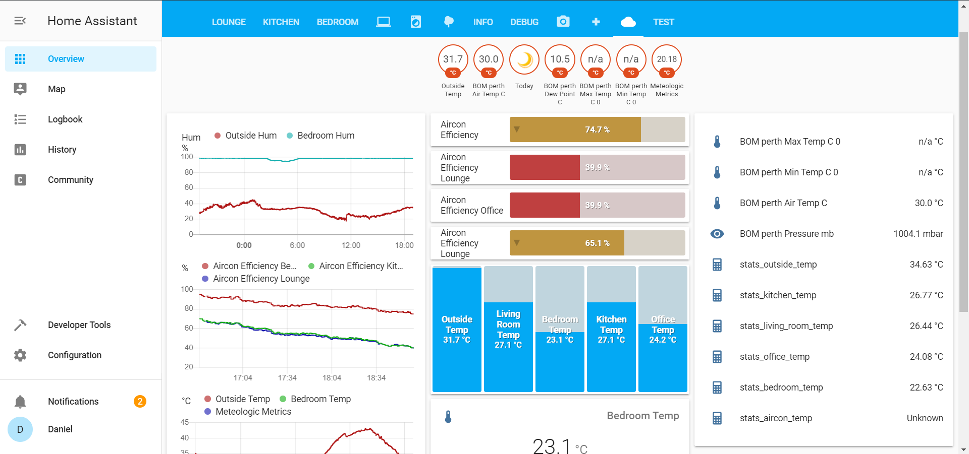
Analysis of current environment
Let’s take a look at the current environment before we begin experiemnting. Right now the indoor temperature is halfway between the other two temperatures, meaning we are operating at roughly 50% efficiency. In other words, $T_{wb} < T_i < T_o$.
The entity card on the right shows current measurements and calculations and confirms that the efficiency is at 45%, meaning there is more cooling potential that can be leveraged..
Now we may say as the outdoor temperature decreases, our efficiency increases as this would close the gap represented by $D_{max}$. This is not true because $T_{wb}$ is determined by the outdoor temperature. meaning a lower outdoor temperature also reduced the wet bulb temperature – maintaining the gap $D_{max}$.
Experiment 1
Let’s run our first eperiment to understand what impact turning on the AC has on the indoor climate. I pressed the “Start experiemnt” button which took a data snapshot and saved it a text file for later analysis.
The following screenshots show the climate dashboards at different intervals. For an explanation of positive or negative efficiency values, check the previous headings.


Climate Dashboard Mid-Experiment at 100% cooling efficiency 

Climate Dashboard Mid-Experiment at 108.7% cooling efficiency 

Climate Dashboard Mid-Experiment at 109% cooling efficiency 

Climate Dashboard Mid-Experiment at 115.1% cooling efficiency
Results

The results of this experiment were great! The graph and table summarises our observations, which were also sent to my phone as a notification.
| Variable | Before | After | Delta | Outcome |
|---|---|---|---|---|
| Efficiency | 45 % | 115.1 % | + 70.1% | Pass – this is clearly a huge improvement |
| Indoor temperature | 28.1 | 21.2 C | – 6.9 C | Pass – we successfully cooled down the house by 6.9 degrees |
| Indoor Humidity | 39.1 | 78.8 % | + 39.7 % | Pass – Humidity increase is expected. its only a problem if we did not reduce the temperature as a result or created excessive humidity causing discomfort. |
Experiment 2: Increasing fan speed from 4 to 8

We can now start an experiment where we increase the fan speed, pushing more hot air through the wet sponges. My hypothesis was that this would not lower the temperature any further because there is less contact time with the sponges.

Counterintuitively, this turned out to be wrong. Faster airflow actually increased the amount of water evaporated, therefore removing more heat energy from the air. Unfortunately, this effect was short lived as $D_{max}$ increased, reducing the margin.
Achieving high efficiency is a sensitive balancing act dependent on many, rapidly changing environmental conditions. Manually adjusting fan speed is therefore not a long term solution and is best handled using some automated method.


I waited a further 5 minutes and Home Assistant reported the results of this experiment which showed a negligible change. The temperature increased by 0.1 C.
Any decrease in temperature would have been cancelled out by the increase in humidity, leaving net zero change to apparent temperature.
| Variable | Before | After | Delta | Outcome |
|---|---|---|---|---|
| Efficiency | 115.1 % | 113 % | – 2.1 | Fail – the adjustment reduced efficiency |
| Indoor temperature | 21.2 C | 21.3 C | +0.1 C | Fail – the adjustment caused an increase in temperature. |
| Indoor Humidity | 78.8 % | 80.5 | + 1.7 % | Pass – Small humidity increase |
This means that slower air rushing through the sponges is able to pick up more moisture, generating a greater cooling effect caused by evaporation.
Conversely, faster moving air deposits more heat energy into the moist sponges, therefore evaporating more water which in turn leads to a higher cooling effect.
Going by by this logic, you might say the best speed is as fast as possible. This is not true either because there is a diminishing effect in the perceived temperature as we are unexessarily increasing the humidity inside the house, negating any additional cooling benefit due to sticky air.
I haven’t fully explored these effects and will need to collect more long term data. It appears there is a tradeoff between good cooling and unecessary increase in humidity. I will keep this in mind going forward to understand how best to optimise around this.
Data driven recommendations
Having integated all these measurements and derived values, I wanted to add smart recommendations to the system. This should tell me whether the AC would be effective at all given the current environmental conditions.
Recommendation 1 (negligle cooling efffect): On a mild but humid day, and an indoor temperature 1 degree above the wet bulb temperature, the system recommends not to turn on the AC because it would vent humid air into the house with negligle reduction in temperature.
This would have the undesired effect of increasing apparent temperature only to squeeze an extra 1 degree of cooling.
Recommendation 2 (indoor conditions already optimal): When AC efficiency is greater than 100%, this means that indoor conditions already exceed the best temperature that can be achieved by evaporative cooling. Turning on the AC would actually increase the temperature and humitity.
Recommendation 3 (aka just open a window): The system detects that the outdoor temperature is lower than inddor temperature. In this scenario the system recommends to turn on the fan to exchange hot indoor air with cooler air from outside. Opening a window in the evening has the same effect.
Conclusion
This project is far from over as I want to build a mathematical model to optimise the variables involved. This problem sounds suspiciously like multivariant optimisation or a classification problem in machine learning.
My next steps include collecting long term data and tuning the sensors to achieve higher accuracy. Any comments or pointers would be appreciated.


